Quick answer: there is no single correct number of bins. Start with a rule of thumb, such as Sturges’ rule (k = ⌈log₂ n⌉ + 1 bins) for small, roughly bell-shaped data or Freedman–Diaconis (width = 2 × IQR × n^(−1/3)) for larger or skewed data. Round the width to something readable, then try a wider and a narrower one. Choose the width at which the shape is clear and stable.
Why the bin width matters
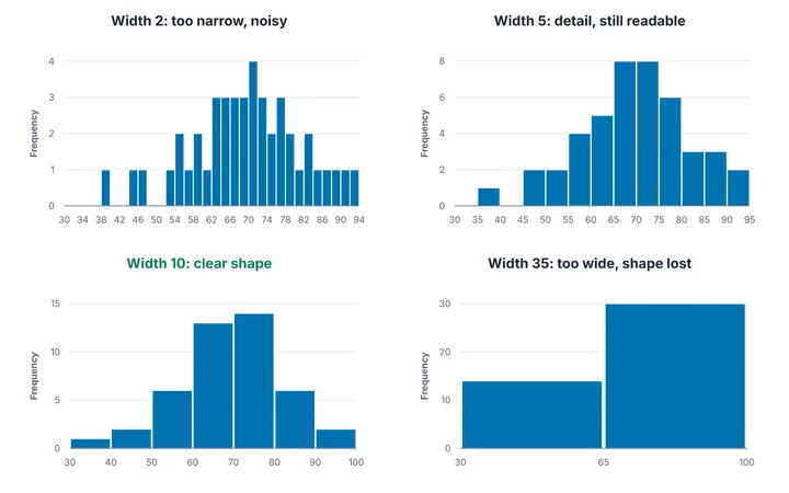
A histogram’s shape depends on how you cut the data into bins. Too narrow and the chart is noisy, with gaps and spikes that come from chance. Too wide and real features, such as two peaks or a long tail, vanish.
The four common rules
Let n be the number of values, s the sample standard deviation, and IQR the interquartile range (Q3 − Q1). The rules give either a number of bins k or a bin width h; they are linked by h = (max − min) ÷ k.
| Rule | Formula | Good for | Weakness |
|---|---|---|---|
| Sturges (Sturges, 1926) | k = ⌈log₂ n⌉ + 1 | Small to medium data that is roughly symmetric | Tends to give too few bins for large or skewed data |
| Square-root | k = ⌈√n⌉ | A quick default; used in some spreadsheet tools | No statistical basis; ignores the spread of the data |
| Scott (Scott, 1979, Biometrika) | h = 3.49 · s · n^(−1/3) | Roughly normal data | Sensitive to outliers because it uses the standard deviation |
| Freedman–Diaconis (Freedman and Diaconis, 1981) | h = 2 · IQR · n^(−1/3) | Skewed data or data with outliers | Can give very narrow bins when the IQR is small |
Note that Sturges and square-root give a number of bins, while Scott and Freedman–Diaconis give a width. You can convert either way with h = (max − min) ÷ k.
A worked example
The histogram maker opens with 44 test scores (sample data). Their summary statistics are:
- n = 44, minimum 38, maximum 94, so the range is 56
- Sample standard deviation s ≈ 12.13
- Q1 = 62 and Q3 = 76.25, so IQR = 14.25
Applying each rule:
| Rule | Calculation | Suggested width |
|---|---|---|
| Sturges | k = ⌈log₂ 44⌉ + 1 = 6 + 1 = 7, so h = 56 ÷ 7 | 8.0 |
| Square-root | k = ⌈√44⌉ = 7, so h = 56 ÷ 7 | 8.0 |
| Scott | h = 3.49 × 12.13 × 44^(−1/3) | 12.0 |
| Freedman–Diaconis | h = 2 × 14.25 × 44^(−1/3) | 8.1 |
The four rules suggest widths from about 8 to 12. All of them round to a readable 10, which gives seven bins from 30 to 100: the “width 10” panel in the picture above. Rounding to a readable width, such as 1, 2, 2.5, 5 or 10 times a power of ten, makes the axis labels easier to read.
How to choose in practice
- Start with a rule. Sturges for small tidy data, Freedman–Diaconis if the data is skewed or large.
- Round to a readable width. Bins from 0 to 10 to 20 are easier to read than 3.7 to 13.9.
- Try one wider and one narrower. If the shape survives, it is probably real. If it changes dramatically, be cautious about conclusions.
- Keep the bin width constant. Equal-width bins let bar height be compared directly.
- State the bin width in the axis title or caption, and which edge belongs to which bin.
Bin edges: which bin does a boundary value belong to?
Conventions differ between programs. In the histogram maker each bin includes its lower edge and excludes its upper edge, except the last bin, which includes both. So a score of exactly 70 is counted in “70 to under 80”, not in “60 to under 70”. Different software can therefore produce slightly different histograms from the same numbers.
Frequently asked questions
How many bins should a histogram have?
Between about 5 and 20 for most data sets, with the exact number depending on the size and shape of your data. Sturges’ rule gives 7 for 44 values and 11 for 1,000 values.
Which rule is the best?
None is best for all data. Sturges is simple and fine for small, symmetric data. Freedman–Diaconis is more robust for skewed data and outliers. Treat any rule as a starting point.
What is density on a histogram’s y-axis?
Density is the count divided by (number of values × bin width), so the total area of the bars is 1. It lets you compare histograms with different bin widths, or overlay a probability curve.
Should I use a histogram or a bar graph?
Use a histogram for one continuous number cut into ranges, and a bar graph for separate categories. See bar graph vs histogram.
References
- Sturges, H. A. (1926). The choice of a class interval. Journal of the American Statistical Association, 21(153), 65–66.
- Scott, D. W. (1979). On optimal and data-based histograms. Biometrika, 66(3), 605–610.
- Freedman, D., and Diaconis, P. (1981). On the histogram as a density estimator: L₂ theory. Zeitschrift für Wahrscheinlichkeitstheorie und verwandte Gebiete, 57, 453–476.
Unfamiliar term? See the chart and graph glossary, or browse the examples gallery.
Spotted an error or something unclear? Tell us and we will fix it. Sources for factual claims are linked in the text. We say so on the page when something is a rule of thumb rather than a standard.