Histogram Maker
Paste raw numbers to get a histogram with automatic bins, a frequency table and summary statistics.
- Free, no account
- Raw numbers in, bins out
- Shows the rule it used
- Data stays in your browser
44 values read. If you use decimal commas, separate numbers with spaces or new lines.
Optional; must not be above your smallest value
7 bins of width 10 (the rule suggests 8.07, rounded to a readable width). Each bin includes its lower edge; the last bin includes its upper edge.
- Count
- 44
- Min
- 38
- Max
- 94
- Mean
- 69
- Median
- 69.5
- Std. dev.
- 12.13
| Bin | Count | Share |
|---|---|---|
| 30 to under 40 | 1 | 2.3% |
| 40 to under 50 | 2 | 4.5% |
| 50 to under 60 | 6 | 13.6% |
| 60 to under 70 | 13 | 29.5% |
| 70 to under 80 | 14 | 31.8% |
| 80 to under 90 | 6 | 13.6% |
| 90 to 100 | 2 | 4.5% |
How to use the histogram maker
- Paste your raw numbers. Separate them with spaces, new lines, commas or semicolons. Every number is one observation, such as one test score or one delivery time. Do not paste counts per category; that is a bar graph.
- Pick a bin rule. Start with the default (Sturges). If your data has a long tail or many points, try Freedman–Diaconis. Or choose a fixed number of bins or a fixed bin width.
- Read the summary. The panel shows the number of bins and their width, the count, minimum, maximum, mean, median and standard deviation, and a table of counts per bin.
- Choose what the Y axis shows. Frequency (count), relative frequency, percent, or density. Use density if bins have different widths or you want to overlay a curve.
- Label and download. Add the variable and its unit as the X axis title, then download a PNG or SVG. The bin table can be copied from the panel.
What you get
- Takes raw valuesYou do not need to count anything first. Paste the data and the tool bins it for you.
- Four automatic rulesSturges, square-root, Scott and Freedman–Diaconis, plus fixed bin count and fixed bin width.
- Shows its workingYou see the bin width the rule suggested, the readable width it rounded to, and every bin’s count and share.
- Summary statisticsCount, min, max, mean, median and sample standard deviation, computed from the numbers you pasted.
- Bars that touch, labels on the edgesBars have no gaps and the axis labels sit on the bin boundaries, as a histogram should.
- Frequency, percent or densitySwitch the Y axis without changing your data.
- Custom starting pointSet where the first bin begins, for example at 0 or at a round number.
Examples: data in, chart out
These charts were made with this tool from the sample data described under each one. Open any of them in the editor to see the exact numbers and settings, or browse the full examples gallery.
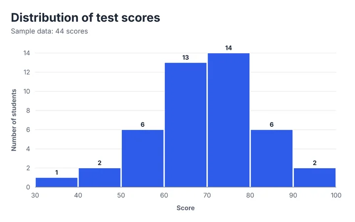
Input: 44 test scores (sample data). Rule: Freedman–Diaconis, which suggests a width of about 8 and is rounded to 10. Result: seven bins from 30 to 100 with most scores between 60 and 80.
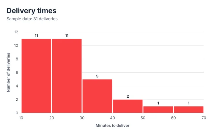
Input: 31 delivery times in minutes (sample data). Rule: Sturges, which suggests about 8.5 and is rounded to 10. Most deliveries fall in the first two bins, and a few slow ones stretch the tail.
How this histogram maker works
Each value is placed in exactly one bin. The bins are equal in width and touch each other.
- Sturges: k = ⌈log₂ n⌉ + 1 bins, so the width is (max − min) ÷ k.
- Square-root: k = ⌈√n⌉ bins.
- Scott: width h = 3.49 · s · n^(−1/3), where s is the sample standard deviation.
- Freedman–Diaconis: h = 2 · IQR · n^(−1/3). Quartiles use linear interpolation (the same as Excel’s QUARTILE.INC and R’s default).
- Readable edges: rule-based widths are rounded to the nearest 1, 2, 2.5 or 5 × 10ⁿ, and the first bin starts at a multiple of that width at or below your smallest value. If you fix the width yourself it is used exactly as typed.
- Edges: each bin includes its lower edge and excludes its upper edge, except the last bin, which includes both. A value equal to a boundary therefore goes into the bin on its right.
- Density is count ÷ (n × bin width), so the bars’ areas add up to 1. Relative frequency is count ÷ n.
Limits you should know about
- Numbers only. Text is skipped and counted, and you are told how many items were skipped.
- Bins are capped at 200. A very small bin width is reduced to fit.
- Equal-width bins only. Variable-width bins are not supported.
- Automatic rules are starting points, not truths. The same data can look different in Excel, R or Python because their defaults and edge conventions differ.
- If your numbers use decimal commas, separate them with spaces or new lines rather than commas.
What happens to your data
The numbers you paste are processed in your browser and autosaved to local storage on this device. Nothing is uploaded. See the privacy notes.
Method last reviewed September 30, 2026. See how we build and check our tools.
When to use it
Exam or test scores
See whether scores cluster, spread out or split into two groups.
Measurements and lab data
Check the shape of repeated measurements before choosing a statistic.
Waiting or delivery times
Reveal a long tail that an average hides.
Quality control
Look at the spread of a part dimension around its target.
Not sure it is a histogram?
Read how a histogram differs from a bar graph.
Choosing the bin width
A worked guide to the rules and their trade-offs.
Tips and common mistakes
- Try more than one bin widthToo few bins hide the shape; too many make it noisy. Change the rule and see whether the story holds.
- Use round bin edgesBins from 0 to 10 to 20 are easier to read than 3.7 to 13.9. Set “First bin starts at” if the automatic start is awkward.
- Label the unitSay “Minutes to deliver” or “Score out of 100” as the X axis title.
- Keep the Y axis at zeroBar height is count. Cutting the axis distorts the shape.
- Do not use a histogram for categoriesColors, countries and product names are categories. Use a bar graph for those.
- Check outliersOne extreme value stretches every bin. The statistics panel shows the min and max to help you spot it.
Frequently asked questions
How do I make a histogram from raw data?
Paste your numbers into the box above, one observation each, separated by spaces, commas or new lines. The tool chooses bins with the rule you select and draws the histogram, a frequency table and summary statistics.
How many bins should a histogram have?
There is no single correct number. Sturges’ rule gives about 1 + log₂(n) bins, which is fine for small, roughly bell-shaped data. Freedman–Diaconis adapts to spread and is often better for larger or skewed data. Try a couple and see whether the shape holds. The bin width guide explains the trade-offs.
What is the difference between a histogram and a bar graph?
A histogram bins one numeric variable into continuous ranges and its bars touch. A bar graph compares separate categories and its bars have gaps. See the full comparison.
Why does my histogram look different from Excel or Google Sheets?
Programs choose their own default bin widths and decide differently which bin a boundary value belongs to. The same numbers can therefore produce differently shaped histograms. Here, each bin includes its lower edge and excludes its upper edge (except the last bin), and you can see and control the bin width.
Which bin does a value on the boundary go into?
The bin on its right. A value of exactly 10 goes into “10 to under 20”, not “0 to under 10”. The last bin includes its upper edge so the maximum is counted.
What does density mean on the Y axis?
Density is count divided by (number of values × bin width). It makes the total area of the bars equal to 1, so histograms with different bin widths can be compared.
Can I set the bin width myself?
Yes. Choose “Fixed bin width” and type the width. You can also choose “Fixed number of bins” and, in either case, set where the first bin starts.
Related chart tools
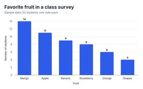
Bar Graph Maker
Vertical, horizontal, grouped and stacked bar graphs from your own data.
Open the tool →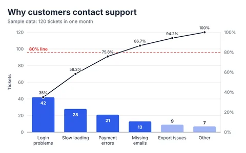
Pareto Chart Maker
Rank causes, add the cumulative line, and find the vital few.
Open the tool →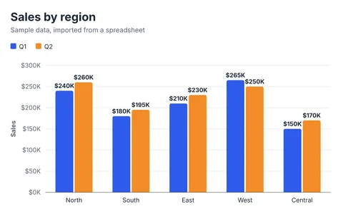
CSV to Bar Chart
Paste from Excel or Google Sheets, or drop a CSV file. Nothing is uploaded.
Open the tool →Guides that go with this tool
- Bar Graph vs Histogram: What's the Difference?A bar graph compares categories; a histogram shows how one number is distributed across ranges. See the differences with examples and how to choose.
- How to Choose a Histogram Bin WidthHow many bins should a histogram have? Compare Sturges, square-root, Scott and Freedman–Diaconis rules, with formulas and a worked example you can check.