Quick answer: in Excel, select your data (labels in one column, numbers in the next), open the Insert tab, choose Insert Column or Bar Chart, and pick Clustered Column (vertical bars) or Clustered Bar (horizontal bars). In Google Sheets, select the data, choose Insert › Chart, and set the chart type to Column chart or Bar chart. Or skip the menus: copy the cells and paste them into the CSV to bar chart tool.
Menu names differ slightly between versions and languages, but the steps below follow the same shape everywhere.
Prepare your data
Both programs expect a simple table:
| Fruit | Students |
|---|---|
| Mango | 14 |
| Apple | 11 |
| Banana | 9 |
- Put the category labels in the first column and the numbers in the next.
- Add a header row with a name for each column. It becomes the legend or axis title.
- Avoid blank rows and merged cells inside the table, and remove any “Total” row before charting, or it will be drawn as another bar.
Make a bar graph in Excel
- Click any cell inside your table (or select the whole range).
- Open the Insert tab.
- In the Charts group, click Insert Column or Bar Chart.
- Choose a type. In Excel’s wording, a column chart has vertical bars and a bar chart has horizontal bars. Pick Clustered Column or Clustered Bar for one or more series side by side, or Stacked Column to stack them.
- Click the chart title and type your own. Use the + (Chart Elements) button beside the chart to add Axis Titles and Data Labels.
- Check the axis. Right-click the vertical axis, choose Format Axis, and confirm the Minimum bound is 0. Excel usually starts column charts at zero, but not always.
- To sort the bars, sort your table first (Data tab › Sort). The chart follows the table.
- To get the chart as an image, click it, copy it (Ctrl+C or Cmd+C) and paste it into a graphics editor or a document, as described in Microsoft’s guide to saving a chart as a picture. Some versions also offer Save as Picture when you right-click the chart.
Microsoft’s own walkthrough, Create a chart from start to finish, covers the Insert tab and chart types in more detail.
Make a bar graph in Google Sheets
- Select your data, including the header row.
- Choose Insert › Chart. Sheets will suggest a type.
- In the Chart editor on the right, under Setup, open Chart type and choose Column chart (vertical) or Bar chart (horizontal). There are also stacked versions.
- Open the Customize tab to add a chart title and axis titles, change colors, and show data labels.
- To download, open the chart’s ⋮ menu and choose Download, then pick PNG, SVG or PDF.
The faster way: paste into a chart maker
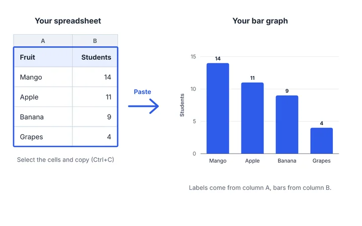
If all you need is a clear, well-labeled image for a document or slide, a chart maker can be quicker:
- Select the cells in Excel or Sheets, including the header row, and copy them (Ctrl+C or Cmd+C).
- Open the bar graph maker and click the first cell of the table, then paste. It reads tabs, thousands separators, currency symbols and percent signs.
- Or export the sheet as CSV (Excel: File › Save As › CSV; Sheets: File › Download › CSV) and drop the file onto the data panel of the CSV to bar chart tool. The file is read in your browser and not uploaded.
- Adjust the design, then download a PNG or SVG.
Which should you use? Charting inside Excel or Sheets is best when the chart must live in the workbook and update when the data changes. A chart maker is quicker when you want a standalone image with good defaults (a zero baseline, sorted bars, alt text) and no account.
Fix the common problems
The bars are in the wrong order. Sort the table. Charts draw categories in the order they appear in the data.
The chart drew a “Total” bar. Remove the total row from the selected range.
The numbers are read as text. If the cells are left-aligned or show a green triangle in Excel, they are stored as text. Convert them to numbers, or paste them into the maker, which parses numbers such as “$1,200” and “12%”.
The axis does not start at zero. Set the minimum manually as in step 6 above. See bar graph best practices for why this matters.
Two columns of numbers gave one bar each. That is a grouped chart, with two bars per category. To stack them instead, choose a stacked type. See types of bar graphs.
Frequently asked questions
What is the difference between a column chart and a bar chart in Excel?
Excel calls a chart with vertical bars a column chart and a chart with horizontal bars a bar chart. Outside Excel, both are usually called bar graphs.
Can I make a bar graph from a CSV file?
Yes. Open the CSV in Excel or Sheets and follow the steps above, or drop it into the CSV to bar chart tool, which builds the chart directly.
Why does my Excel chart look different from the one here?
Different programs use different defaults for gaps, fonts, colors and axis scaling. In the maker you can control the gap width, palette, font and axis in the Design tab.
Unfamiliar term? See the chart and graph glossary, or browse the examples gallery.
Spotted an error or something unclear? Tell us and we will fix it. Sources for factual claims are linked in the text. We say so on the page when something is a rule of thumb rather than a standard.